Evaluation Test Number 4 (practice 3)
Contents
Exercise 1. a
If Y(t) is the solution of the following Initial Value Problem (IVP)


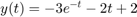
our final goal is to obtain the value Y (1.2) by solving numerically the IVP. a) Check that the function 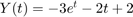 is the solution of this IVP. It is not necessary to deduce it, but only substitute it in the ODE. In general, an analytical expression of the solution like this is not known, but in academic exercises this situation is used to check the goodness of the numerical methods.
Answer:
 (1)
(1)
derivative: 
substituting (1) in diferential equation:
 (2)
(2)

 (3)
(3)
we check that (2) = (3)
Exercise 1. b
Apply the Euler method for h = 0.05, h = 0.1, h = 0.2 and h = 0.4. Plot from t = 0 to t = 1.2 in the same picture: the exact solution and the solutions obtained for these four values of h. Discuss what you see in this picture.
Functions used:
function [t,y] = eulode(dydt,tspan,y0,h,varargin)
%   eulode: Euler ODE solver
%   [t,y] = eulode(dydt,tspan,y0,h,p1,p2,...):
%           uses Euler's method to integrate an ODE
%   input:
%   dydt = name of the M-file that evaluates the ODE
%   tspan = [ti, tf] where ti and tf = initial and
%   final values of independent variable
%   y0 = initial value of dependent variable
%   h = step size
%   p1,p2,... = additional parameters used by dydt
%   output:
%   t = vector of independent variable
%   y = vector of solution for dependent variable
if nargin<4,error('at least 4 input arguments required'),end
ti = tspan(1);tf = tspan(2);
if ~(tf>ti),error('upper limit must be greater than lower'),end
t = (ti:h:tf)'; n = length(t);
% if necessary, add an additional value of t
% so that range goes from t = ti to tf
if t(n)<tf
   t(n+1) = tf;
   n = n+1;
end
y = y0*ones(n,1); %preallocate y to improve efficiency
for i = 1:n-1 %implement Euler's method
   y(i+1) = y(i) + dydt(t(i),y(i),varargin{:})*(t(i+1)-t(i));
end
clear, clf
ti= 0;
tf= 1.2;
h = [0.05 0.1 0.2 0.4];
colour='brgc';
tspan=[0 1.2];
y0= -1;
t=ti:h(1):tf;
yt= -3*exp(-t) - 2*t +2;  % y exact true
plot(t,yt,'-');
hold on;
dydt = @(t,y) (-2*t -y);
i=1;
while i <= length(h)
    [t1,ye]=eulode(dydt,tspan,y0,h(i));
    argcol=strcat('--',colour(i));
    plot(t1,ye,argcol);
    hold on;
    i=i+1;
end
legend('exact','h=0.05','h=0.1','h=0.2','h=0.4');
title('Euler Method');
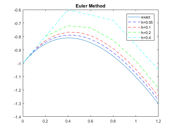
Discussion:
Exercise 1. c
Compute and plot the same as b) but applying the fourth-order Runge-Kutta (RK4) method. Discuss now what you see in this picture.
Functions used:
function [tp,yp] = rk4sys(dydt,tspan,y0,h,varargin)
% rk4sys: fourth-order Runge-Kutta for a system of ODEs
%   [t,y] = rk4sys(dydt,tspan,y0,h,p1,p2,...): integrates
%           a system of ODEs with fourth-order RK method
% input:
%   dydt = name of the M-file that evaluates the ODEs
%   tspan = [ti, tf]; initial and final times with output
%           generated at interval of h, or
%   = [t0 t1 ... tf]; specific times where solution output
%   y0 = initial values of dependent variables
%   h = step size
%   p1,p2,... = additional parameters used by dydt
% output:
%   tp = vector of independent variable
%   yp = vector of solution for dependent variables
if nargin<4,error('at least 4 input arguments required'), end
if any(diff(tspan)<=0),error('tspan not ascending order'), end
n = length(tspan);
ti = tspan(1);tf = tspan(n);
if n == 2
  t = (ti:h:tf)'; n = length(t);
  if t(n)<tf
    t(n+1) = tf;
    n = n+1;
  end
else
  t = tspan;
end
tt = ti; y(1,:) = y0;
np = 1; tp(np) = tt; yp(np,:) = y(1,:);
i=1;
while(1)
  tend = t(np+1);
  hh = t(np+1) - t(np);
  if hh>h,hh = h;end
  while(1)
    if tt+hh>tend,hh = tend-tt;end
    k1 = dydt(tt,y(i,:),varargin{:})';
    ymid = y(i,:) + k1.*hh./2;
    k2 = dydt(tt+hh/2,ymid,varargin{:})';
    ymid = y(i,:) + k2*hh/2;
    k3 = dydt(tt+hh/2,ymid,varargin{:})';
    yend = y(i,:) + k3*hh;
    k4 = dydt(tt+hh,yend,varargin{:})';
    phi = (k1+2*(k2+k3)+k4)/6;
    y(i+1,:) = y(i,:) + phi*hh;
    tt = tt+hh;
    i=i+1;
    if tt>=tend,break,end
  end
  np = np+1; tp(np) = tt; yp(np,:) = y(i,:);
  if tt>=tf,break,end
end
clear, clf
ti= 0;
tf= 1.2;
h = [0.05 0.1 0.2 0.4];
colour='brgc';
tspan=[0 1.2];
y0= -1;
t=ti:h(1):tf;
yt= -3*exp(-t) - 2*t +2;  % y exact true
plot(t,yt,'-');
hold on;
dydt = @(t,y) (-2*t -y);
i=1;
while i <= length(h)
    [t1,ye]=rk4sys(dydt,tspan,y0,h(i));
    argcol=strcat('--',colour(i));
    plot(t1,ye,argcol);
    hold on;
    i=i+1;
end
legend('exact','h=0.05','h=0.1','h=0.2','h=0.4');
title('RK4 Method');
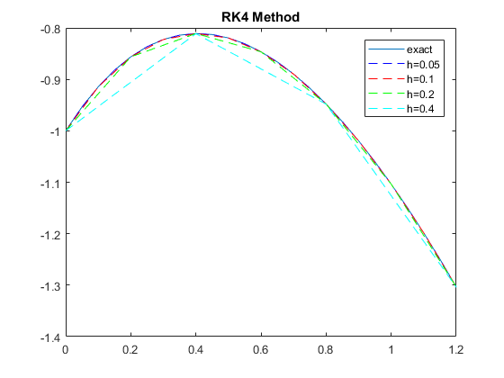
Discussion:
Exercise 1. d
Fill in the following table for the step size h = 0.2, where  and
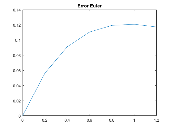
and  are the numerical solutions by Euler and RK4 method respectively and
 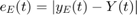 ,
,  their errors.
Functions used: eulode, rk4sys
clear;
clc;
format long;
h=0.2;
y0 = -1;
tspan=[0 1.2];
t=0:h:1.2;
yt= -3*exp(-t)-2*t+2;
dydt = @(t,y) (-2*t -y);
[t,yE] = eulode(dydt,tspan,y0,h);
[t,yRK4] = rk4sys(dydt,tspan,y0,h);
eE=abs(yE - yt');
eRK4 = abs(yRK4 - yt');
pr=[t; yt; yE'; yRK4'; eE'; eRK4'];
fprintf('ti       Y(ti)       yE(ti)      yRK4(ti)      eE(ti)    eRK4(ti)\n');
fprintf('%3.1f  %10.8f  %10.8f  %10.8f  %10.4e  %10.4e\n',pr);
figure;
plot(t,eE');title('Error Euler');
figure;
plot(t,eRK4');title('Error RK4');
ti       Y(ti)       yE(ti)      yRK4(ti)      eE(ti)    eRK4(ti)
0.0  -1.00000000  -1.00000000  -1.00000000  0.0000e+00  0.0000e+00
0.2  -0.85619226  -0.80000000  -0.85620000  5.6192e-02  7.7408e-06
0.4  -0.81096014  -0.72000000  -0.81097281  9.0960e-02  1.2675e-05
0.6  -0.84643491  -0.73600000  -0.84645047  1.1043e-01  1.5566e-05
0.8  -0.94798689  -0.82880000  -0.94800389  1.1919e-01  1.6993e-05
1.0  -1.10363832  -0.98304000  -1.10365571  1.2060e-01  1.7391e-05
1.2  -1.30358264  -1.18643200  -1.30359972  1.1715e-01  1.7086e-05
Discussion:
Exercise 1. e
We define as  and
and 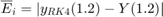 the final errors in t = 1.2 when the step hi is used for Euler and RK4 method respectively. Fill in the following table with errors
  and
and  and their rates
  and
and  :
:
Functions used: eulode, rk4sys
clear;
clc;
format long;
h = [0.4 0.2 0.1 0.05 0.025 0.0125];
hf = 1.2;
Y= -3*exp(-hf)-2*hf+2;
y0 = -1;
tspan=[0 1.2];
% t=0:h:1.2;
dydt = @(t,y) (-2*t -y);
fprintf('i     h        E(i)        r(i)         Erk(i)       rrk(i)\n');
E=[];
Erk=[];
for i=0:length(h)-1
    [t,yE] = eulode(dydt,tspan,y0,h(i+1));
    [t,yRK4] = rk4sys(dydt,tspan,y0,h(i+1));
    E(i+1) = abs(yE(end) - Y);
    Erk(i+1) = abs(yRK4(end) - Y);

    if  i == 0
        pr=[i; h(i+1); E(i+1);  Erk(i+1)];
        fprintf('%1d  %6.4f  %10.5e       -       %10.5e      -\n',pr);
    else
        ri = E(i+1)/E(i);
        rpi= Erk(i+1)/Erk(i);
        pr=[i; h(i+1); E(i+1); ri; Erk(i+1); rpi];
        fprintf('%1d  %6.4f  %10.5e  %10.5e  %10.5e  %10.5e\n',pr);
    end
end
i     h        E(i)        r(i)         Erk(i)       rrk(i)
0  0.4000  2.55583e-01       -       3.23369e-04      -
1  0.2000  1.17151e-01  4.58367e-01  1.70861e-05  5.28379e-02
2  0.1000  5.62940e-02  4.80527e-01  9.82205e-07  5.74855e-02
3  0.0500  2.76156e-02  4.90559e-01  5.88782e-08  5.99449e-02
4  0.0250  1.36794e-02  4.95349e-01  3.60395e-09  6.12103e-02
5  0.0125  6.80810e-03  4.97692e-01  2.22911e-10  6.18520e-02
Discussion:
Exercise 1. f
If we assume that, for a step  , the global error for a numerical method of order p is
  where C is a constant does not depend on , justify the values that appear as
  and
and  .
.
Discussion:
Exercise 2. a
Consider the problem of an orbit of a satellite, whose position and velocity are obtained as the solution of the following state equation:
x'1(t) = x3(t)
x'2(t) = x4(t)
x3'(t) = -G M x1(t)=(x^21(t) + x^22(t))^3/2
x4'(t) = -G M x2(t)=(x^21(t) + x^22(t))^3/2
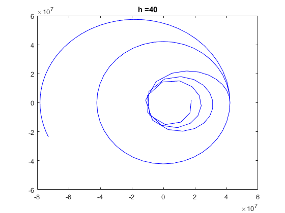
where G = 6.672 . 10^-11 N m2/kg2 is the gravitational constant and M = 5.97 . 10^24 kg is the mass of the earth. Note that (x1, x2) and (x3, x4) denote the position and velocity, respectively of the satellite on the plane having the earth at its origin. Use RK4 method with step h = 40, h = 400 and h = 1728 to find the paths of the satellite with the following initial positions/velocities for one day
- i) (x1, x2) = (4.223 . 10^7, 0) [m] and (x3, x4) = (0, 2000) [m/s]
- ii) (x1, x2) = (4.223 . 10^7, 0) [m] and (x3, x4) = (0, 3071) [m/s]
- iii) (x1, x2) = (4.223 . 10^7, 0) [m] and (x3, x4) = (0, 3500) [m/s]
a) For each value of h, plot on the plane (x1, x2) the three paths for satellite in the same picture and deliver it. Comment the differences than can appear between the three values of h.
Functions used:
function dx=df_sat(t,x)
global G Me Re
dx=zeros(size(x));
r=sqrt(sum(x(1:2).^2));
if r<=Re,
    return;
end % when colliding against the Earth surface
GMr3=G*Me/r^3;
dx(1)=x(3); dx(2)=x(4); dx(3)= -GMr3*x(1); dx(4)= -GMr3*x(2);
function [t,y]=ode_RK4(f,tspan,y0,N,varargin)
%Runge-Kutta method to solve vector differential equation y'(t)=f(t,y(t))
% for tspan=[t0,tf] and with the initial value y0 and N time steps
if nargin<4|N<=0, N=100; end
if nargin<3, y0=0; end
y0=y0(:)'; %make it a row vector
y=zeros(N+1,length(y0)); y(1,:)=y0;
h=(tspan(2)-tspan(1))/N;
t=tspan(1)+[0:N]'*h;
h2=h/2;
for k=1:N
  %if y(k,1)<0, pause; end
  f1=h*feval(f,t(k),y(k,:),varargin{:}); f1=f1(:)'; %(6.3-2a)
  f2=h*feval(f,t(k)+h2,y(k,:)+f1/2,varargin{:}); f2=f2(:)';%(6.3-2b)
  f3=h*feval(f,t(k)+h2,y(k,:)+f2/2,varargin{:}); f3=f3(:)';%(6.3-2c)
  f4=h*feval(f,t(k)+h,y(k,:)+f3,varargin{:}); f4=f4(:)'; %(6.3-2d)
  y(k+1,:)= y(k,:) +(f1+2*(f2+f3)+f4)/6; %Eq.(6.3-1)
end
clear, clf
global G Me Re
G = 6.672e-11; Me = 5.97e24; Re = 64e5;
t0 = 0; T = 24*60*60; % Time in sec. for a day
tf = T;
tspan=[0 tf];
h = [40 400 1728];
R = 4.223e7;  % distance of satellite from center of earth
v20s = [2000 3071 3500];
for i=1:length(h)
    for iter = 1:length(v20s)
        x10 = R; x20 = 0; v10 = 0; v20 = v20s(iter);
        x0 = [x10 x20 v10 v20];
        [tR,xR] = ode_RK4(@df_sat,tspan,x0,h(i));
        plot(xR(:,1),xR(:,2),'b');
        hold on;
    end
    tit=strcat('h = ',num2str(h(i)));
    title(tit);
    figure;
end


Discussion:
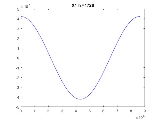
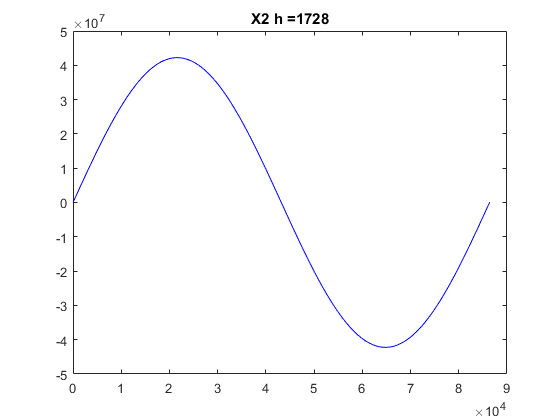
Exercise 2. b
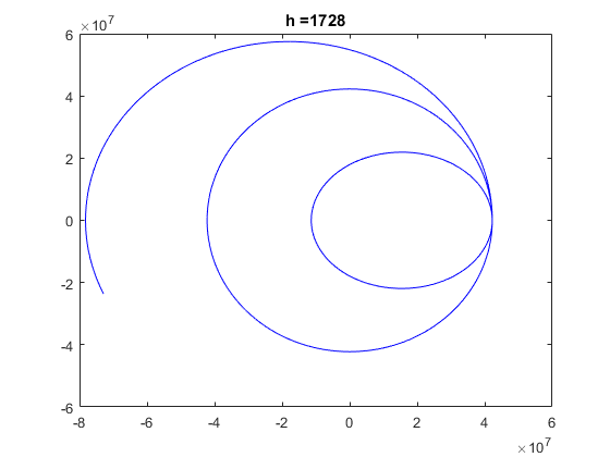
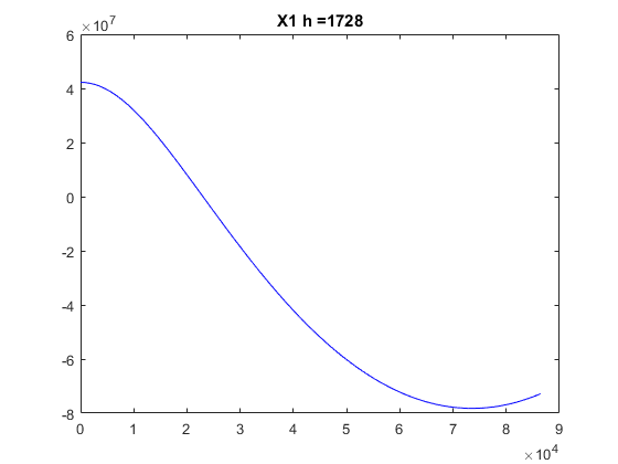
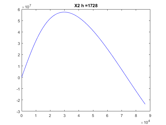
b) Choose the value h you prefer and plot only the position x1 along a day in the three cases (in the same picture o not, as you want). Plot the position x2 in the three cases in another picture.
Functions used: df_sat, ode_RK4
clear, clf
global G Me Re
G = 6.672e-11; Me = 5.97e24; Re = 64e5;
t0 = 0; T = 24*60*60; % Time in sec. for a day
tf = T;
tspan=[0 tf];
h = [40 400 1728];
R = 4.223e7;  % distance of satellite from center of earth
v20s = [2000 3071 3500];
for iter = 1:length(v20s)
    x10 = R; x20 = 0; v10 = 0; v20 = v20s(iter);
    x0 = [x10 x20 v10 v20];
    [tR,xR] = ode_RK4(@df_sat,tspan,x0,h(3));
    plot(tR,xR(:,1),'b');
    tit=strcat('X1 h = ',num2str(h(3)));
    title(tit);
    hold on;
end
figure;
for iter = 1:length(v20s)
    x10 = R; x20 = 0; v10 = 0; v20 = v20s(iter);
    x0 = [x10 x20 v10 v20];
    [tR,xR] = ode_RK4(@df_sat,tspan,x0,h(3));
    plot(tR,xR(:,2),'b');
    tit=strcat('X2 h = ',num2str(h(3)));
    title(tit);
    hold on;
end
Discussion:
Exercise 2. c
c) How many half rounds does the satellite travel in a day? You can answer simply looking at the previous pictures, for example. But it is necessary to justify the answer.
Justification:
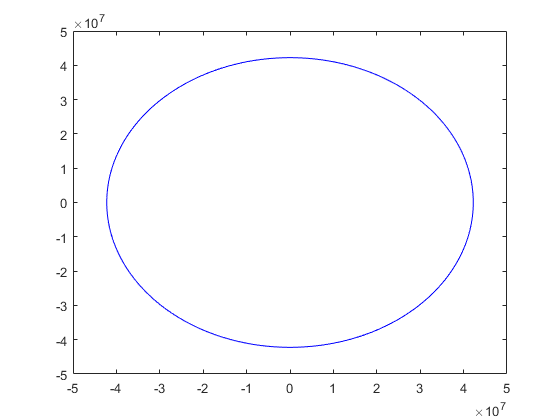
Exercise 2. d
d) At what time is the satellite back to the starting point when the initial condition is ii)?
clear, clf
global G Me Re
G = 6.672e-11; Me = 5.97e24; Re = 64e5;
t0 = 0; T = 24*60*60; % Time in sec. for a day
tf = T;
tspan=[0 tf];
h = [40 400 1728];
R = 4.223e7;  % distance of satellite from center of earth
v20s = [2000 3071 3500];
x10 = R; x20 = 0; v10 = 0; v20 = v20s(2);
x0 = [x10 x20 v10 v20];
[tR,xR] = ode_RK4(@df_sat,tspan,x0,h(3));
plot(xR(:,1),xR(:,2),'b');
figure;
plot(tR,xR(:,1),'b');
tit=strcat('X1 h = ',num2str(h(3)));
title(tit);
hold on;
figure;
x10 = R; x20 = 0; v10 = 0; v20 = v20s(2);
x0 = [x10 x20 v10 v20];
[tR,xR] = ode_RK4(@df_sat,tspan,x0,h(3));
plot(tR,xR(:,2),'b');
tit=strcat('X2 h = ',num2str(h(3)));
title(tit);
hold on;
Answer:
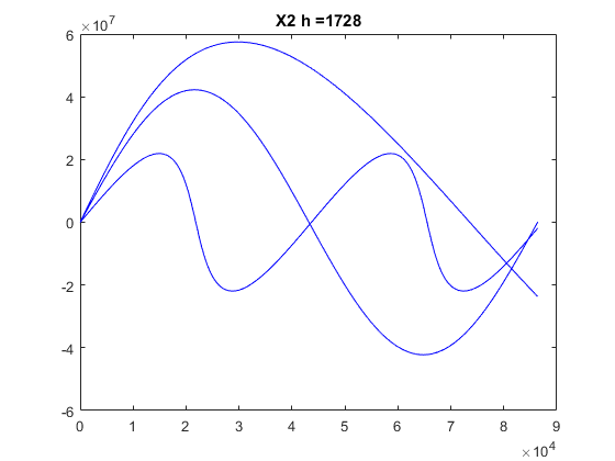
Exercise 2. e
e) At what time is the satellite back to the starting point when the initial condition is iii)?
clear, clf
global G Me Re
G = 6.672e-11; Me = 5.97e24; Re = 64e5;
t0 = 0; T = 24*60*60; % Time in sec. for a day
tf = T;
tspan=[0 tf];
h = [40 400 1728];
R = 4.223e7;  % distance of satellite from center of earth
v20s = [2000 3071 3500];
x10 = R; x20 = 0; v10 = 0; v20 = v20s(3);
x0 = [x10 x20 v10 v20];
[tR,xR] = ode_RK4(@df_sat,tspan,x0,h(3));
plot(tR,xR(:,1),'b');
tit=strcat('X1 h = ',num2str(h(3)));
title(tit);
figure;
x10 = R; x20 = 0; v10 = 0; v20 = v20s(3);
x0 = [x10 x20 v10 v20];
[tR,xR] = ode_RK4(@df_sat,tspan,x0,h(3));
plot(tR,xR(:,2),'b');
tit=strcat('X2 h = ',num2str(h(3)));
title(tit);
Answer: